SimpleCrop

SimpleCrop.jl is a compact, executable crop model assembled from phenology, canopy, biomass partitioning, weather, and soil-water components. This tutorial follows the short integration case in Cropbox's test/examples/simplecrop.jl, then reads its output from the perspective of the crop as a whole.

SimpleCrop follows the intentionally simplified model in the official DSSAT teaching material, A Modular Approach to Structure Crop Models. It is useful for learning how components exchange values and how a complete simulation is organized; it is not a fully parameterized production model.

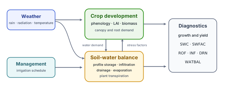
Weather and management supply the environment. Crop development, canopy, biomass, and below-ground water balance advance together, while diagnostic variables expose the resulting state.

Load the example inputs

Add the model and the table-reading packages to your active Julia environment:

using Pkg
Pkg.add(["Cropbox", "SimpleCrop", "CSV", "DataFrames"])

The package test data contain daily weather and irrigation tables. Run the remaining blocks in order in the same session.

using Cropbox
using SimpleCrop
using CSV
using DataFrames

loaddata(name) = CSV.File(
    joinpath(dirname(pathof(SimpleCrop)), "../test/data", name)
) |> DataFrame

weather = loaddata("weather.csv")
irrigation = loaddata("irrigation.csv")

(weather = first(weather, 3), irrigation = first(irrigation, 3))

(weather = 3×6 DataFrame
 Row │ DATE (:Date)  SRAD (MJ/m^2/d)  TMAX (°C)  TMIN (°C)  RAIN (mm/d)  PAR ( ⋯
     │ Date          Float64          Float64    Float64    Float64      Float ⋯
─────┼──────────────────────────────────────────────────────────────────────────
   1 │ 1986-01-01                6.3       22.8       13.9         22.6        ⋯
   2 │ 1986-01-02                6.3       20.6       12.8          0.0
   3 │ 1986-01-03                6.2       20.6       13.3          0.3
                                                                1 column omitted, irrigation = 3×2 DataFrame
 Row │ DATE (:Date)  IRR (mm/d) 
     │ Date          Int64      
─────┼──────────────────────────
   1 │ 1986-01-01             0
   2 │ 1986-01-02             0
   3 │ 1986-01-03             0)

The annotated CSV headers retain dates, units, and column types. Cropbox normalizes them when the corresponding provide and drive variables are constructed.

Configure and run the model

config = @config (
    Clock => :step => 1u"d",
    Calendar => :init => ZonedDateTime(1987, 1, 1, tz"UTC"),
    SimpleCrop.Weather => :weather_data => weather,
    SimpleCrop.SoilWater => :irrigation_data => irrigation,
)

result = simulate(SimpleCrop.Model;
    config,
    stop = :endsim,
)

(rows = nrow(result), start = first(result.DATE), finish = last(result.DATE))

(rows = 294, start = Date("1987-01-01"), finish = Date("1987-10-21"))

This is the same execution path exercised by the framework test. :endsim is a flag declared by the model, so the biological state rather than a hard-coded number of days determines when the run stops.

Read development and canopy growth

N is leaf number and LAI is leaf area index. They provide a quick check that phenology and canopy development are advancing together.

visualize(result,
    :DATE,
    [:N, :LAI];
    kind = :line,
)

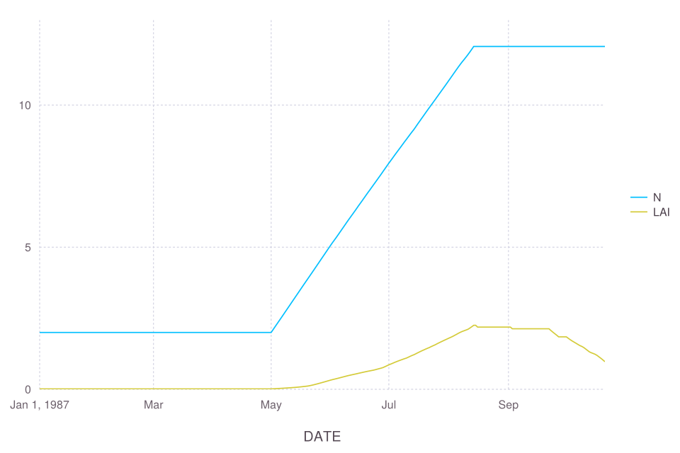
The test suite plots LAI; displaying N beside it adds the developmental context needed to interpret the canopy trajectory.

Read biomass partitioning

W is total dry biomass. The component pools Wc, Wr, and Wf represent canopy, root, and fruit biomass.

visualize(result,
    :DATE,
    [:W, :Wc, :Wr, :Wf];
    names = ["Total", "Canopy", "Root", "Fruit"],
    kind = :line,
)

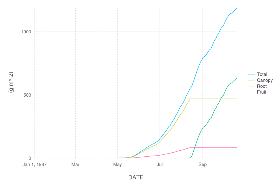
Read these curves together with development and LAI: a change in allocation is part of the crop's developmental program, not just a final yield calculation.

Check one coupled environmental state

The integration test also plots stored soil water SWC divided by profile depth DP.

visualize(result,
    :DATE,
    :(SWC / DP);
    yunit = u"mm^3/mm^3",
    kind = :line,
)

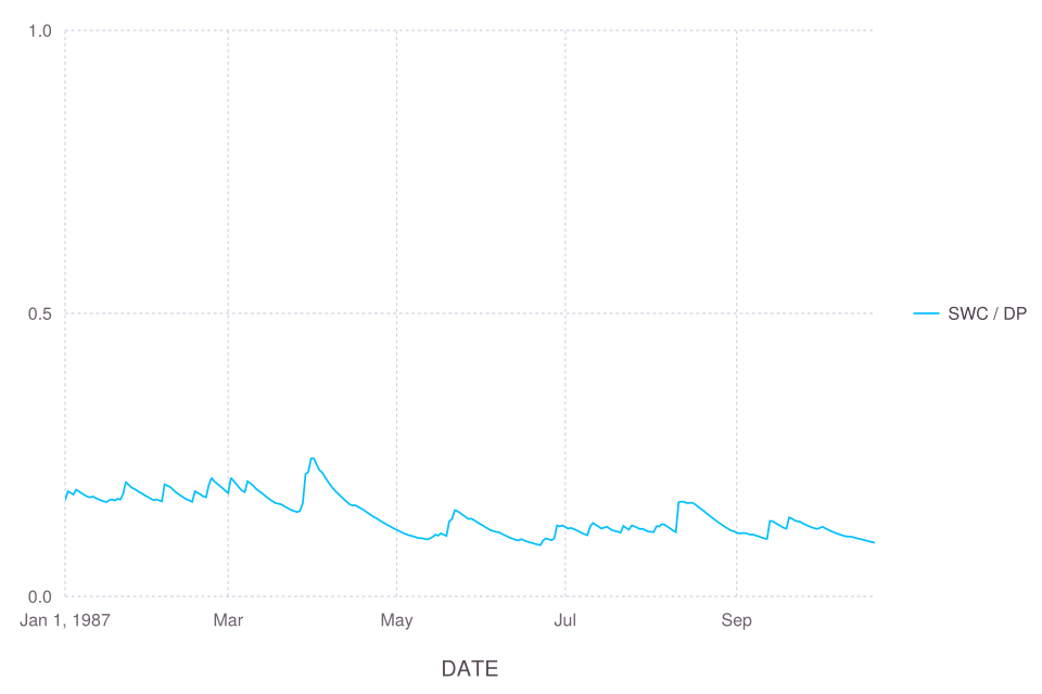
This plot confirms that the environmental component is connected and evolving during the crop run. It is not intended as a stand-alone validation of a layered soil-water algorithm. For the separate multi-layer implementation in Cropbox's own test suite, continue with Soil Water Transport.

What this example establishes

The short test demonstrates the complete integration path:

1. tabular weather and management data enter through configuration;
2. a daily clock advances all model components;
3. phenology, canopy, biomass, and environmental states remain coupled;
4. a model-declared flag stops the simulation; and
5. the resulting table can be inspected or visualized without model-specific plotting code.

Use the model's own repository for cultivar parameters and scientific changes. Use Cropbox's configuration, simulation, and visualization pages for framework-level options.